T&C LAB-AI
Dept. of Intelligent Robot Eng. MU
Robotics
Optimization Method
Lecture 4
Jeong-Yean Yang
2020/10/22
1
T&C LAB-AI
Dept. of Intelligent Robot Eng. MU
Robotics
Optimization
• Optimization Definition
– Find parameters,w for minimizing scalar function, J.
• Cost(Scalar ,Objective) function
– Define J and try to minimize it
– J= scalar function
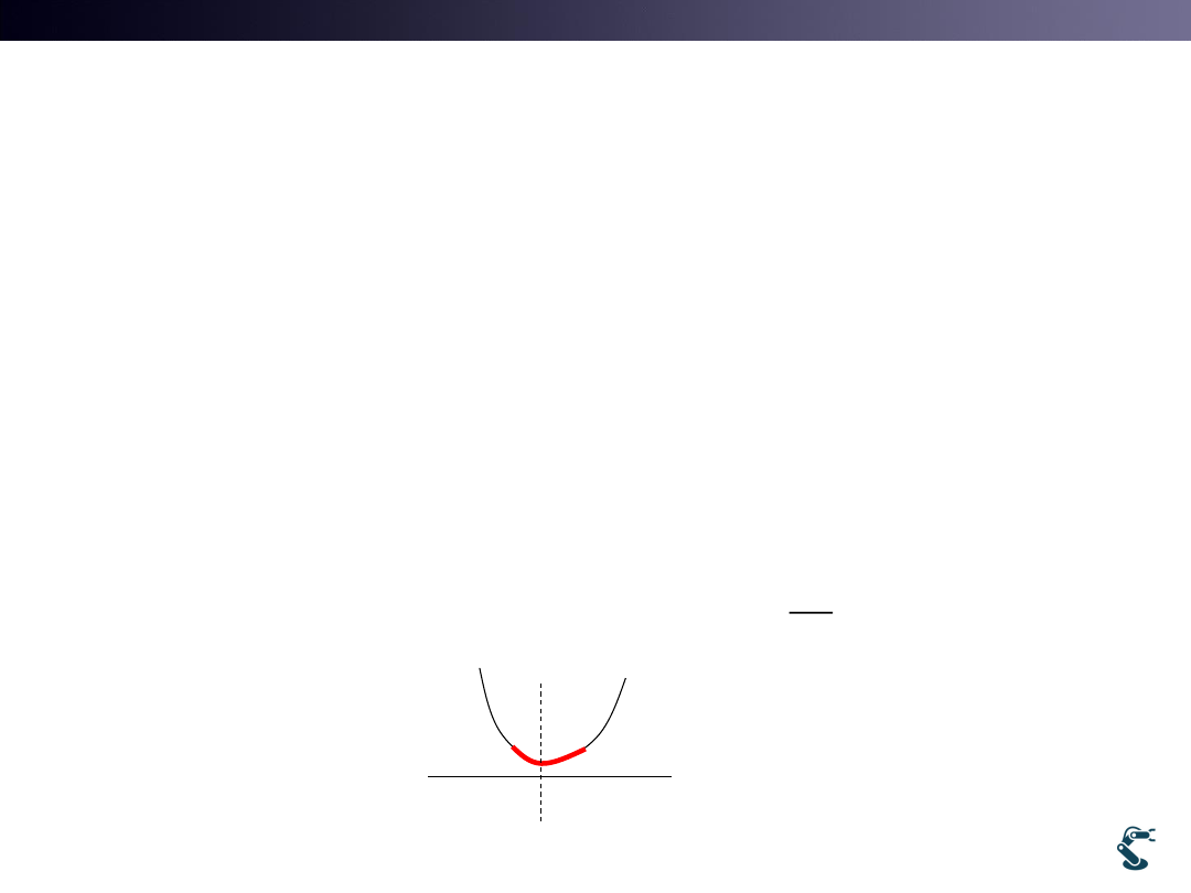
• J Must be Convex Hull
– Convex(볼록) Vs. Concave(오목)
– At a Convex hull, Differentiation is zero
2
Convex
( ), :
J
J
Parameter
0
J
w
J
w
w*
T&C LAB-AI
Dept. of Intelligent Robot Eng. MU
Robotics
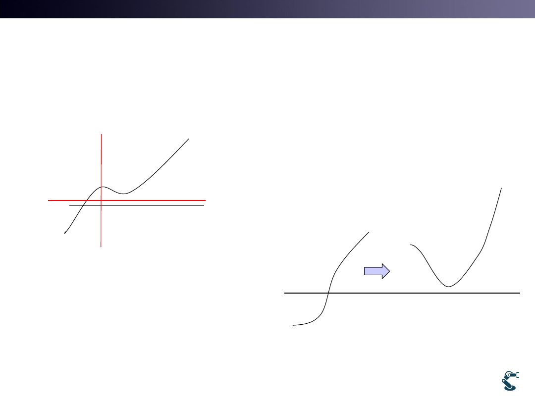
If My Cost Function has No Convex Hull,..
3
• 2. Use Square
– Ex) Minimum Squared Error
• 1. Constraint is needed
• Constraints
– Equality constraint
– Inequality constraint
J
w
2
( )
new
J
J
J
J
2
J
J
, min
?
J
c
J
J
a
w
b
, min
?
J
a
J
T&C LAB-AI
Dept. of Intelligent Robot Eng. MU
Robotics
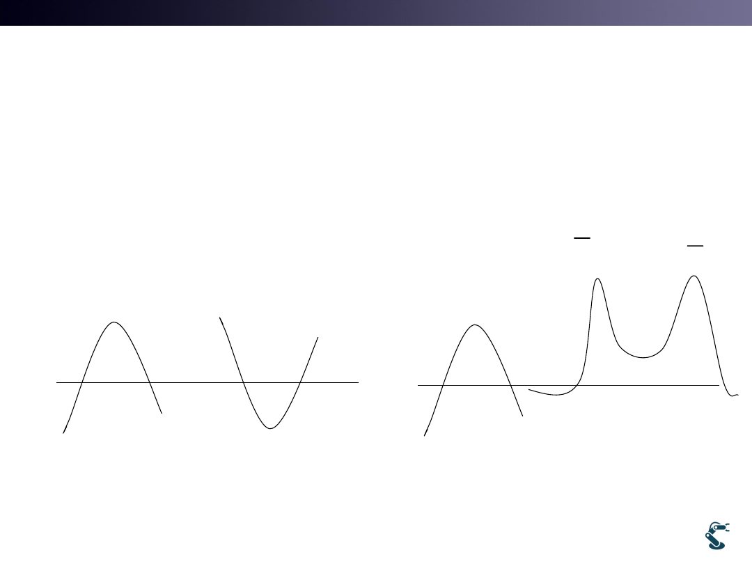
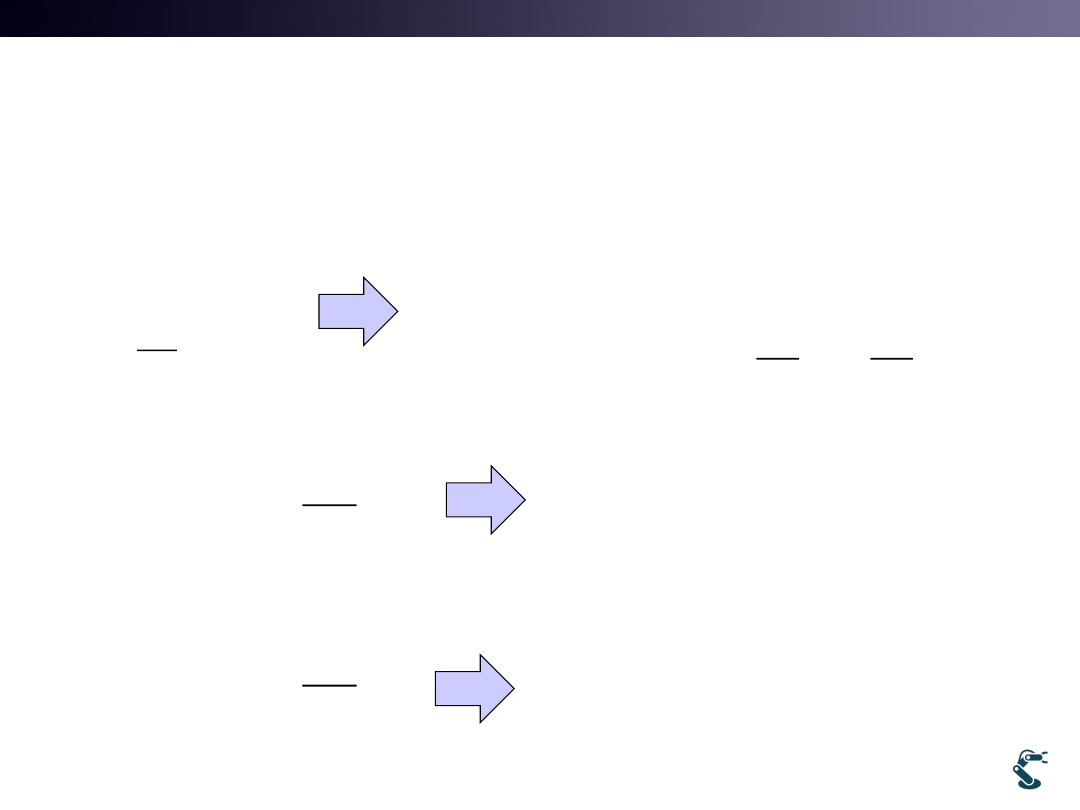
If My J has Maximum Convex Hull,…
• Use Minus
4
• 2. Use Denomination
J
( )
new
J
J
J
J
J’=-J
( )
1
new
J
J
J
J
J
1
J
T&C LAB-AI
Dept. of Intelligent Robot Eng. MU
Robotics
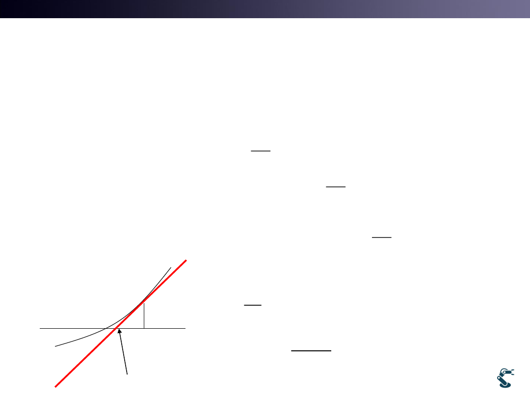
What We learn in Last Week
• 1.Differentiation=0
– Case 1) Linear equation
– Case 2) Non-Linear equation
•
Non-Linear Newton-Raphson Method
5
( )
0
J
J
J
w
( , )
( )
J(a, b)
0,
0
w
a b
J
J
J
J
a
b
0
i
J
w
Aw
b
0
i
J
w
( )
0
( )
0
f w
g w
T&C LAB-AI
Dept. of Intelligent Robot Eng. MU
Robotics
Simple Optimization
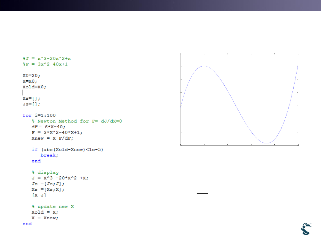
• How to do optimization?
• We know Minimum exists where
• Think Newton Method again, f(x)=0
6
( )
J
J
0
J
w
0
J
w
1
(
)
( )
0
'( )
i
i
i
i
i
i
f
y
x
x
f x
x
f x
x
x
x
f x
Xi
Xi+1
( )
0
J
f x
w
T&C LAB-AI
Dept. of Intelligent Robot Eng. MU
Robotics
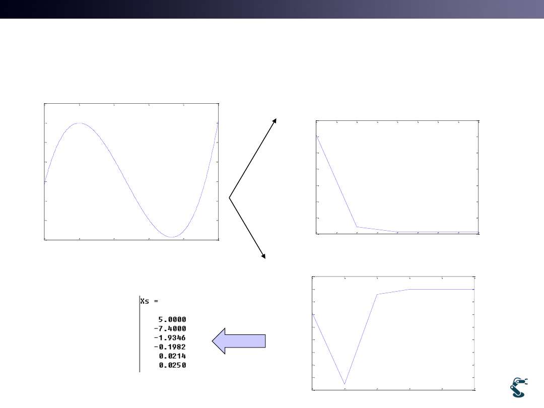
Ex) Optimization with Newton Method
Test1.m xxxxxx
7
-5
0
5
10
15
20
-1200
-1000
-800
-600
-400
-200
0
200
x
y
J=x
3-20x2+x
minJ with x>=0
3
2
20
J
x
x
x
2
3
40
1
0
'
6
40
J
F
x
x
x
F
x
T&C LAB-AI
Dept. of Intelligent Robot Eng. MU
Robotics
1
2
3
4
5
6
-1600
-1400
-1200
-1000
-800
-600
-400
-200
0
200
Iteration
J
X0=5
1
1.5
2
2.5
3
3.5
4
4.5
5
-1200
-1000
-800
-600
-400
-200
0
200
Iteration
J
X0=20
Effect of First Guess Value
8
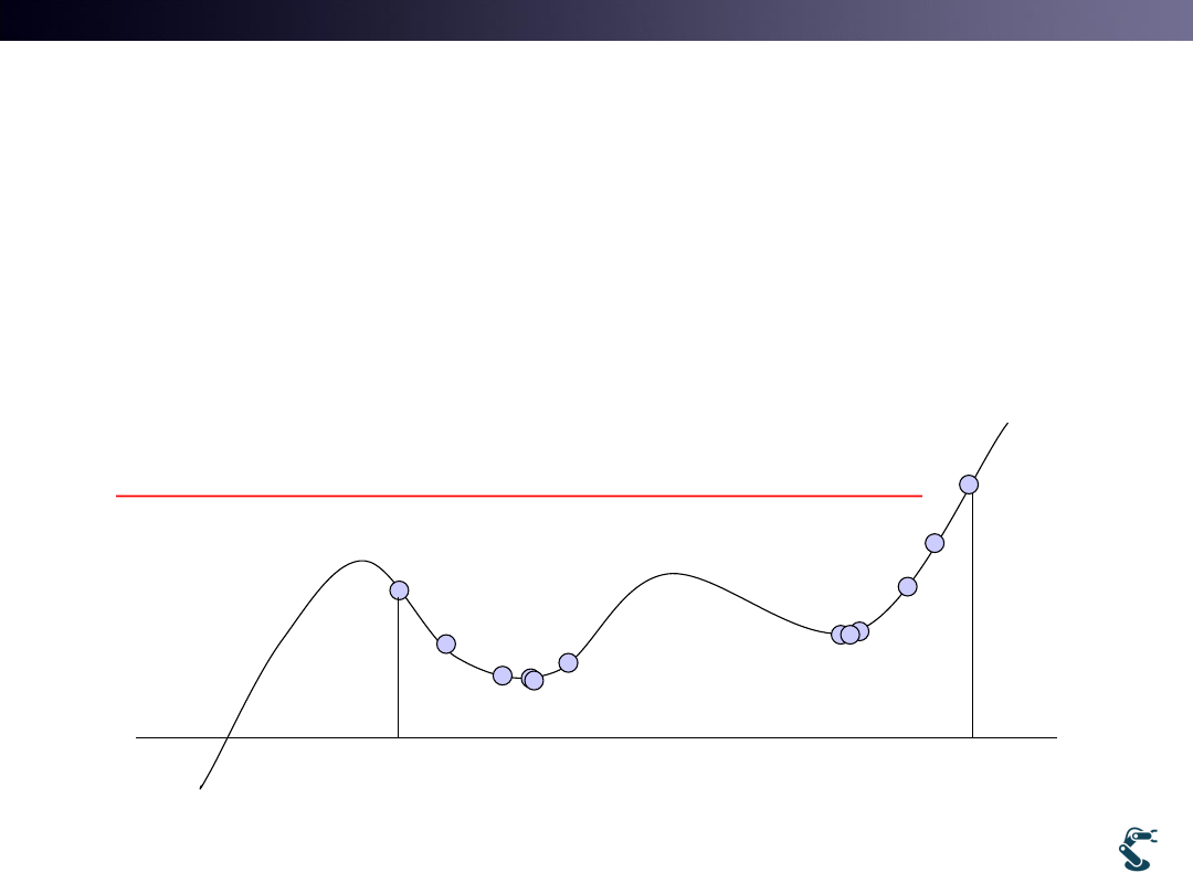
• Start with X0=5 Xmin=0.025
• Start with X0=20 Xmin=13.3
-5
0
5
10
15
20
-1200
-1000
-800
-600
-400
-200
0
200
x
y
J=x
3-20x2+x
minJ with x>=0
3
2
20
J
x
x
x
T&C LAB-AI
Dept. of Intelligent Robot Eng. MU
Robotics
Guess with Multiple Minimum(=Minima)
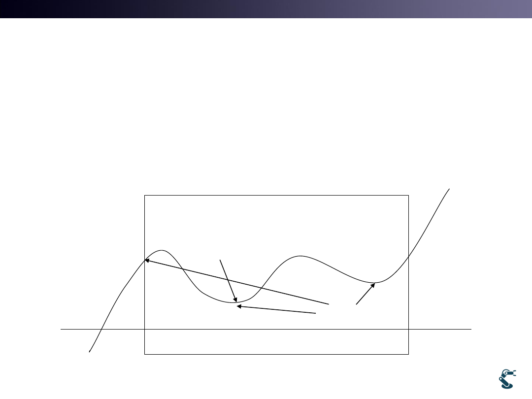
• Where You Start?
• Solution Highly Depends on Initial Guess.
– Keep it “If there are More than One Minimum”
9
x0
x0
Iterative Method depends on the Initial Guess
Because the Method is finding
Local Minima
T&C LAB-AI
Dept. of Intelligent Robot Eng. MU
Robotics
Guess with Multiple Minimum(=Minima)
• Where You Start?
• Solution Highly Depends on Initial Guess.
– Keep it “there are More than one Minimum”
10
1. Constraint =?
Local Minima
Global Minimum:
Minimum of
Minima

T&C LAB-AI
Dept. of Intelligent Robot Eng. MU
Robotics
Optimization with Differentiation
in a Multi Dimensional Vector Space
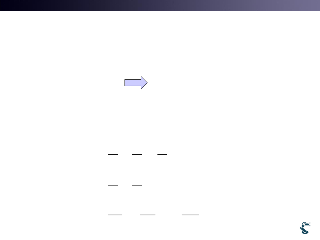
• Differentiation is the KEY for Any Equation in Any Space
• You learned Differentiation in Function Space
– Function Space : a set of functions from a set X to a set Y
– Function : X F(X)=Y
• Well, Differentiation in a Multi dimensional Vector Space?
– You have used Differentiation with X and Y in the Vector Space!!
11
( )
( )
( )
( )
'( )
y
f x
f x
dy
df x
dx
x
dy
f x
f x
dx
x
T&C LAB-AI
Dept. of Intelligent Robot Eng. MU
Robotics
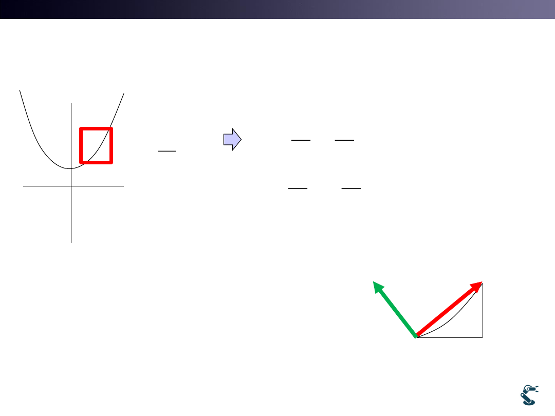
Gradient Definition:
Differentiation in a Multidimensional Vector Space
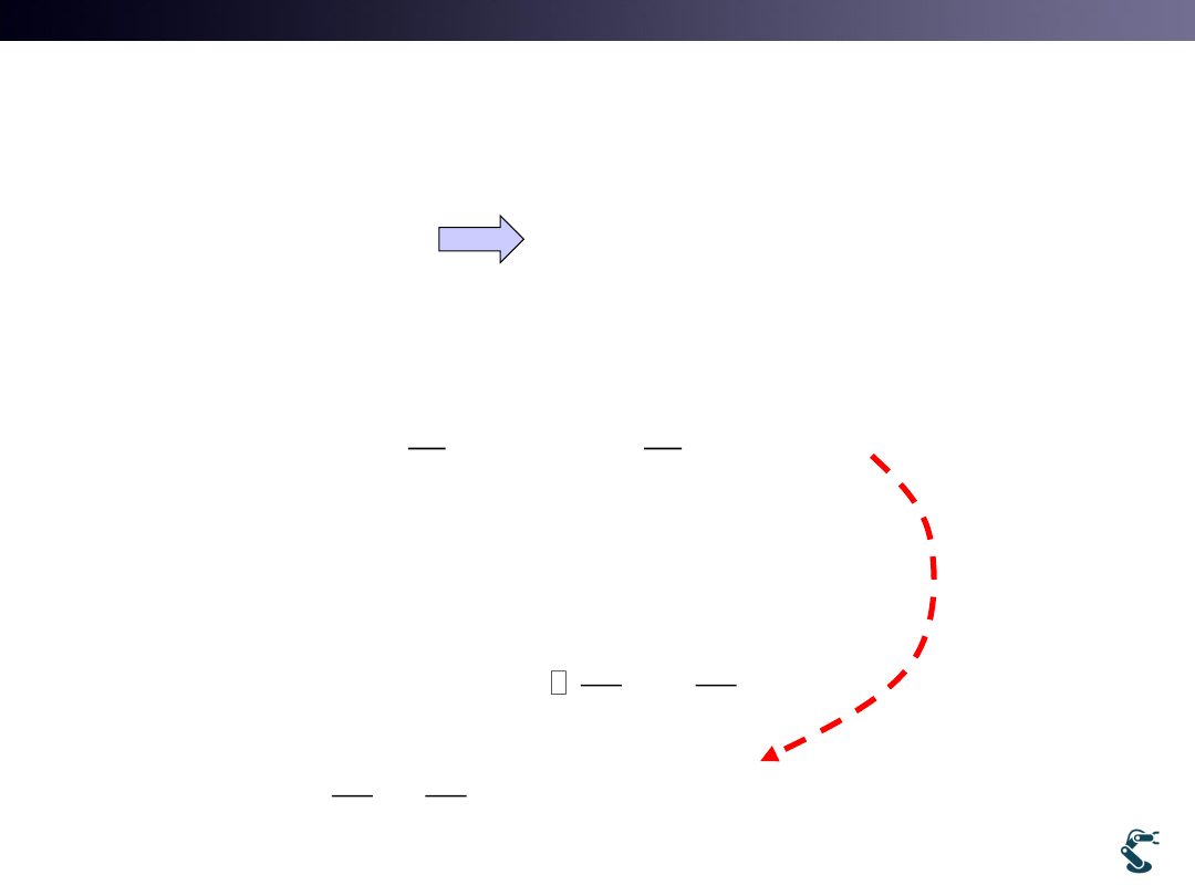
• Y=F(x) is a function. In other words,
• How we do Differentiation in a x,y vector space?
• Define Gradient
12
( )
y
f x
( , )
( )
0
g x y
y
f x
Function
Equation
ˆ
ˆ
ˆ
Grad
i
j
k
x
y
z
x,y,z space
ˆ
ˆ
Grad
i
j
x
y
x,y space
1
2
1
2
ˆ
ˆ
ˆ
...
N
N
Grad
n
n
n
w
w
w
N space
Neural
Network
T&C LAB-AI
Dept. of Intelligent Robot Eng. MU
Robotics
Function Vs. Equation
• Use Gradient,
• Use Total derivative
13
( )
y
f x
( , )
( )
0
g x y
y
f x
Function
Equation
ˆ
ˆ
( , )
(
( ))
(
( ))
ˆ ˆ
'( )
g x y
y
f x i
y
f x j
x
y
f x i
j
. . of g
( , )
ˆ
ˆ
ˆ
ˆ
ˆ
g
g
T D
dg x y
dx
dy
x
y
g
g
dg
i
j
dxi
dyj
g dX
x
y
T&C LAB-AI
Dept. of Intelligent Robot Eng. MU
Robotics
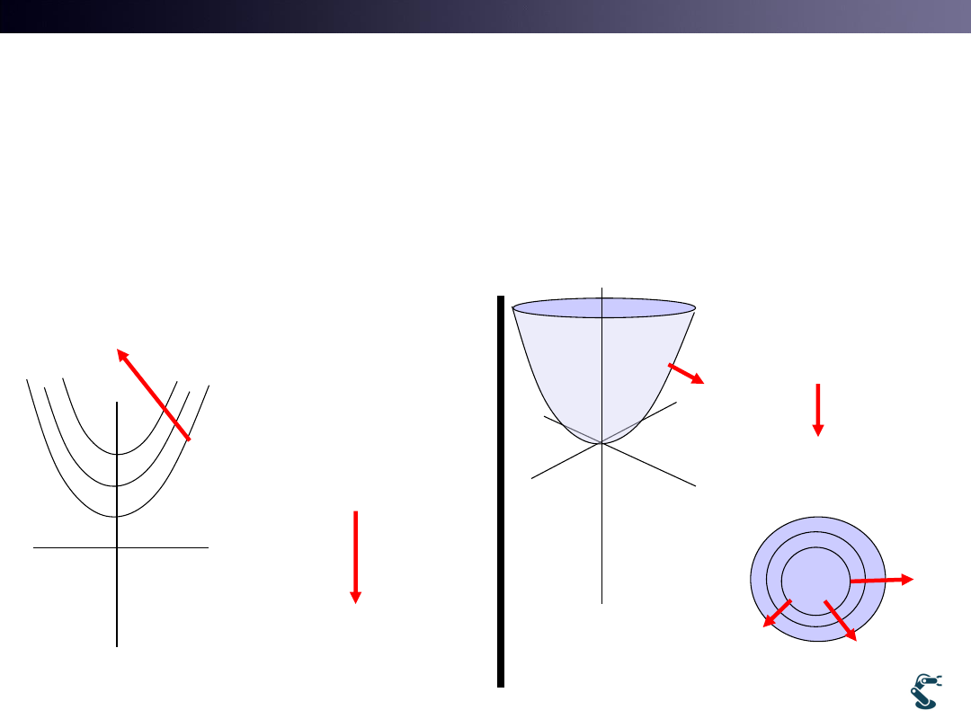
Gradient: Normal Vector
• Focus on that
• Gradient is a Normal Vector to a vector
14
2
1
y
x
2
dy
x
dx
2
( , )
1
0
ˆ
ˆ
ˆ
ˆ
2
1
ˆ
2
0
g x y
y
x
g
g
g
i
j
xi
j
x
y
g
g
dg
dx
dy
g dX
xdx
dy
x
y
ˆ
0
ˆ
dg
g dX
g
dX
ˆ
dX
dx
dy
ˆ
dX
g
T&C LAB-AI
Dept. of Intelligent Robot Eng. MU
Robotics
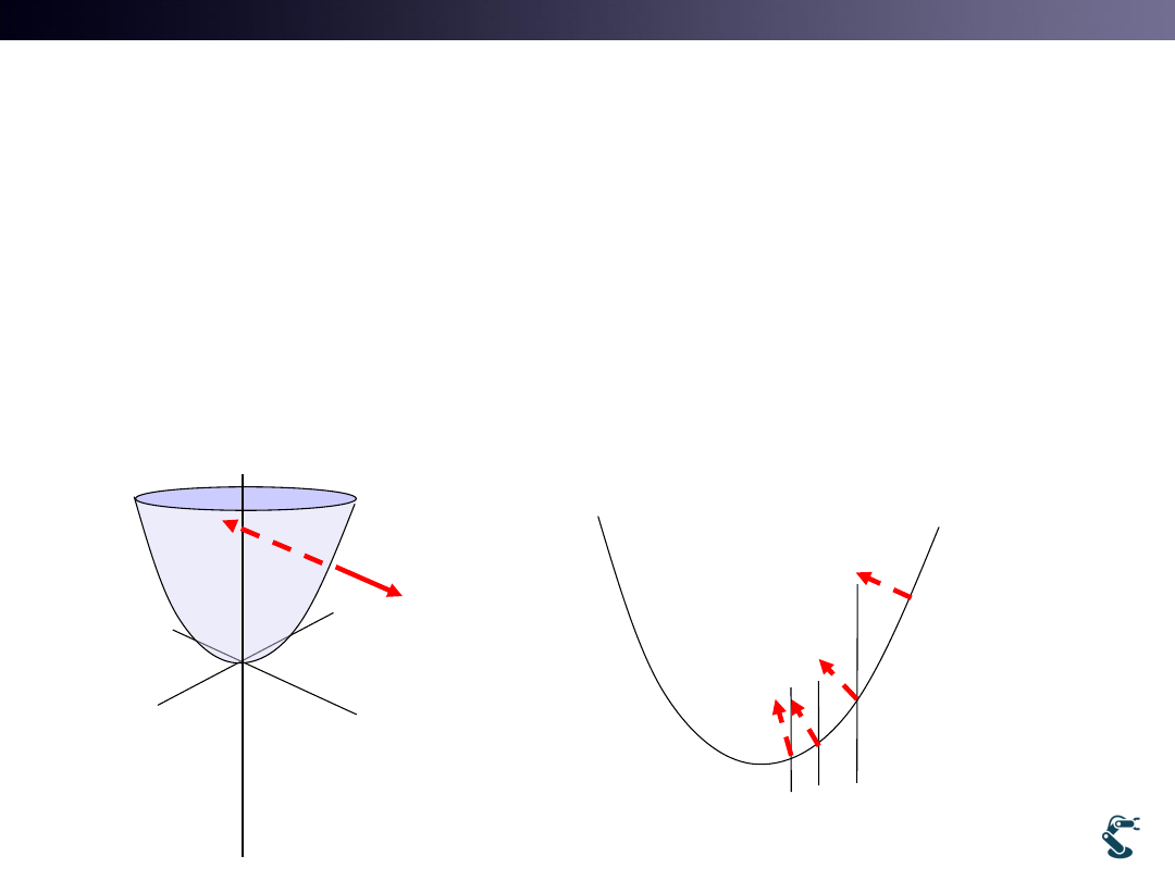
Gradient Direction
• Gradient Direction
– The Greatest Rate of Function Increment
15
2
2
1
1
y
x
g
y
x
2
2
2
( , )
1
0
( , )
1 1
( , )
1
2
...
g x y
y
x
g x y
y
x
g x y
y
x
Function
Increment
Function
Increment
g
2
2
2
2
2
2
( , )
1
( , )
2
( , )
3
...
g x y
x
y
g x y
x
y
g x y
x
y
g
Function
Increment
T&C LAB-AI
Dept. of Intelligent Robot Eng. MU
Robotics
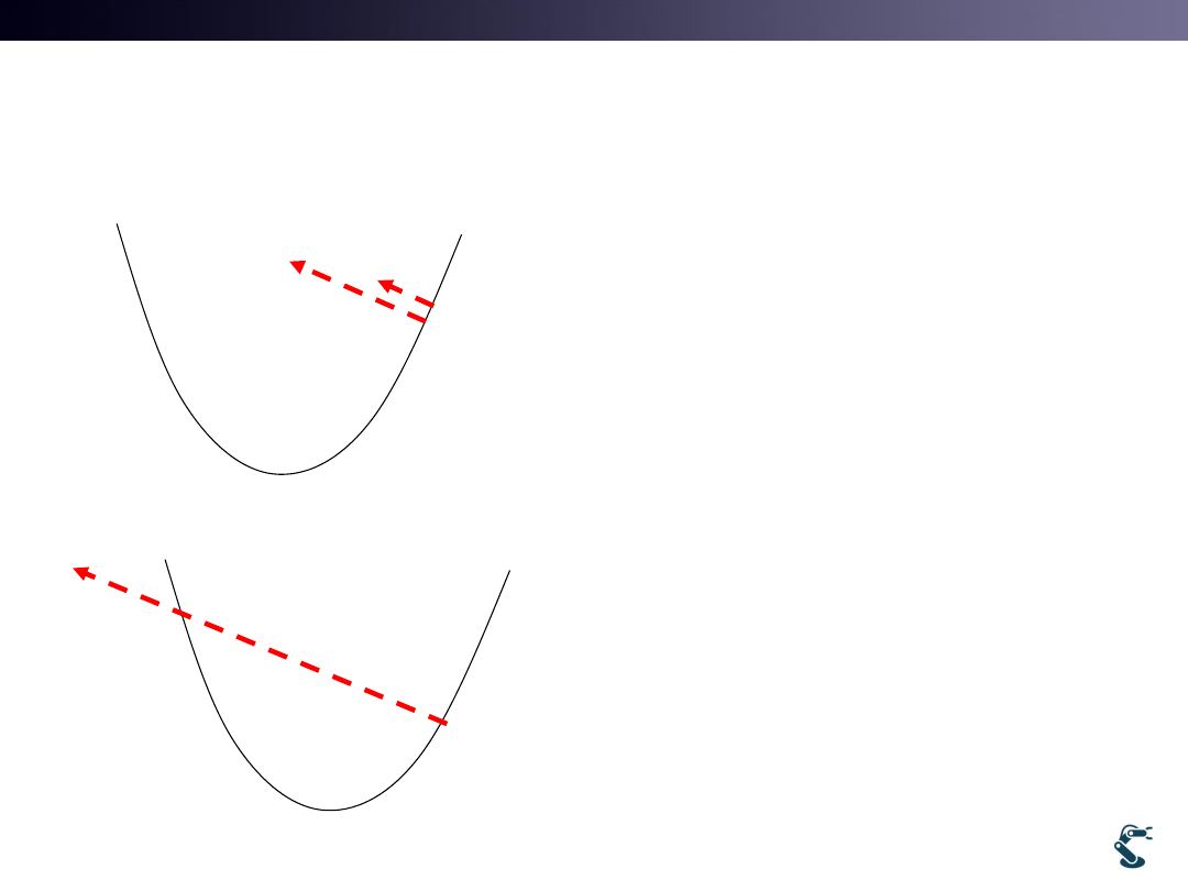
Optimization with Gradient
• Gradient Direction = Function Increment
• Optimization = Find Function Minimum
Optimization = Reverse Direction of Gradient ?
16
g
g
g
Focus on that
Minus Gradient
Direction is
changing.
At the minima,
Minus Gradient
direction sees
top
T&C LAB-AI
Dept. of Intelligent Robot Eng. MU
Robotics
Gradient Descent Method I
• Gradient Descent
• How far we go?
– With Alpha scalar..
• Small alpha
– It could be a Long Journey
– Too many iterations
• Big alpha
– It passes minima.
– Solution becomes unstable.
17
g
g
g
g
g
Big alpha passes minima

T&C LAB-AI
Dept. of Intelligent Robot Eng. MU
Robotics
Gradient Descent Method II
• 1. Guess X = X0
• 2. Calculate Next Point
• 3. Check Stop Condition
• 4. Go to 2
18
1
n
n
X
X
g
1
|
|
, stop
|
|
n
n
n
X
X
if
X
T&C LAB-AI
Dept. of Intelligent Robot Eng. MU
Robotics
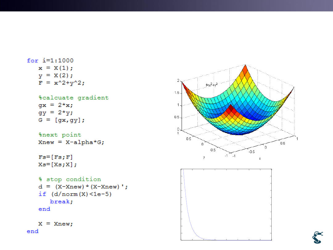
GDM Example (test2.m)
19
2
2
( , )
f x y
x
y
0
5
10
15
20
25
30
35
40
0
0.2
0.4
0.6
0.8
1
1.2
1.4
1.6
1.8
2
Iteration
F(
x
,y
)
Alpha=0.1
T&C LAB-AI
Dept. of Intelligent Robot Eng. MU
Robotics
0
10
20
30
40
0
0.5
1
1.5
2
Iteration
F
alpha=0.1
0
50
100
150
200
250
0
0.5
1
1.5
2
Iteration
F
alpha=0.01
0
5
10
15
20
25
0
0.5
1
1.5
2
Iteration
F
alpha=0.2
0
200
400
600
800
1000
0
0.5
1
1.5
2
Iteration
F
alpha=0.5
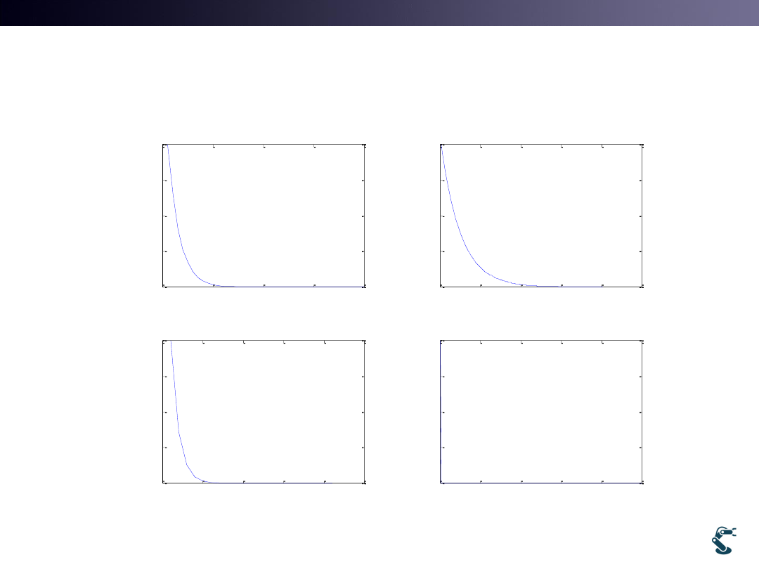
Effect of Alpha(Learning Rate)
20
Diverge!
Small alpha takes
much time
Big alpha becomes
unstable